LTI System

LTI system이란 (1) Linear하고, (2) Time-Invariant한 시스템이다. Linear system은 additivity와 homogeneity가 성립하는 시스템을 뜻한다. Time-Invariant란 입력 신호의 time shift가 출력 신호에 그대로 반영되는 시스템 특성을 의미한다. Time-Invariant system은 시간이 흘러도 시스템 특성이 변하지 않는다.

Convolution Integral

신호 및 시스템 수업에서 배운 것처럼, 어떤 시간 t에서의 입력 신호는 t 이후의 모든 시간에서의 출력 신호에 영향을 줄 수 있다. 따라서 출력은 입력과 impulse response의 convolution integral로 나타낼 수 있다.

Laplace Transform

Convolution integral은 대수적으로 풀기 어렵기 때문에, time-domain에서 convolution integral을 풀기보다는 Laplace transform을 통해 s-domain에서 두 함수의 대수곱으로 변형하여 푼다.

Laplace Transform은 다음과 같이 정의할 수 있다.

\[\mathscr{L} \{ f(t)\}(s)=\int_{0-}^{\infty}f(t)e^{-st}dt\]

Laplace Transform은 f(t)에서 주파수 s인 신호의 진폭과 위상을 얻는 방법이다. Fouries Transform은 s=jw인 Laplace Transform의 특수한 경우이다.

Laplace Transform은 time-domain에서의 컨볼루션 곱을 s-domain에서의 대수곱으로 변형할 수 있다.

\[\mathscr{L}\{f(t)*g(t)\}(s)=\mathscr{L}\{f(t)\}\cdot\mathscr{L}\{g(t)\}\]

Obtaining System Response

시스템 응답을 얻는 과정은 다음과 같다.

1. 전달함수 H(s)를 구한다. \(H(s)=\mathscr{L}\{h(t)\}(s)\), h(t): impulse response
2. 입력 신호 U(s)를 결정한다.
3. 출력 신호를 구한다. \(Y(s)=H(s)U(s)\)
4. Time-domain에서의 출력을 구한다. \(y(t)=\mathscr{L}^{-1}\{Y(s)\}\)

Transfer Function

Transfer function이란 s-domain에서 입력 신호와 출력 신호의 비이다. Time-domain differential equation으로부터 구할 수도 있고, impulse response를 Laplace Transform하여 구할 수도 있다.

Linear system의 Transfer function은 분모의 차수가 분자의 차수보다 크거나 같은 유리함수로 나타나며, 현실 세계에 존재하는 시스템에 대한 transfer function은 모두 실수 계수를 가진다.

Transfer function을 통해 시스템의 특성을 파악할 수 있는데, 가장 먼저 알아야 할 것이 바로 pole과 zero이다. Pole은 분모를 0으로 만드는 s 값을, Zero는 분자를 0으로 만드는 s 값을 의미한다.

주어진 Transfer function은 다음과 같이 인수분해할 수 있다. \(H(s)=K\frac{\prod_{i=1}^m(s-z_{i})}{\prod_{i=1}^n(s-p_{i})}\). \(p_i\)는 pole을, \(z_{i}\)는 zero를 나타낸다. 만약 \(p_{i}=z_{j}\)인 i, j가 존재한다면 약분해야만 시스템 응답을 제대로 분석할 수 있는데, 우리는 그러한 i, j가 존재하지 않는다고 가정한다. 모델링의 관점에서 보면, \(p_{i}=z_{j}\)인 i, j가 존재하더라도 실제로는 \(p_{i}\not=z_{j}\)임에도 모델링 오차에 의해 pole-zero cancellation을 진행하면 시스템 응답을 제대로 분석할 수 없기 때문이다. 물론 pole에 가까운 zero는 그 pole의 영향을 줄이는 효과가 있지만 응답에 오차가 생기는 것은 사실이다.

아래에서 보겠지만 zero보다는 pole이 응답에 더 큰 영향을 미친다. 특히 s-plane에서 pole이 imaginary axis 상에 있다면 neutral stable하고 pole이 ORHP에 있다면 시스템 응답이 발산하기에, 우리는 pole이 OLHP상에 있는 상황을 가정한다.

\(s=-\sigma\pm j\omega_{d}\)를 pole로 가지는 second-order transfer function을 고려하자.

\(H(s)=\frac{\sigma^{2}+\omega_{d}^{2}}{(s+\sigma)^{2}+\omega_{d}^{2}}\), \(\omega_{n}^{2}=\omega_{d}^{2}+\sigma^{2}, \zeta=\tan^{-1}\left(\frac{\sigma}{\omega_{n}}\right)\)로 정의하면

\(H(s)=\frac{\omega_{n}^{2}}{s^{2}+2\zeta\omega_{n}+\omega_{n}^{2}}\)으로 쓸 수 있고, 식을 풀면 \(h(t)=1-e^{-\zeta\omega_{n}t}\left(\cos\omega_{d}t+\frac{\sigma}{\omega_{d}}\sin\omega_{d}t\right)\)로 쓸 수 있다. 여기서 \(\zeta\)를 damping ratio라 하고, 감쇠/진동의 정도를 나타낸다. h(t)에서 exponential term이 감쇠항, cos & sin term이 진동항이다. damping ratio가 클수록 감쇠의 정도가 심하다.

Block Diagram

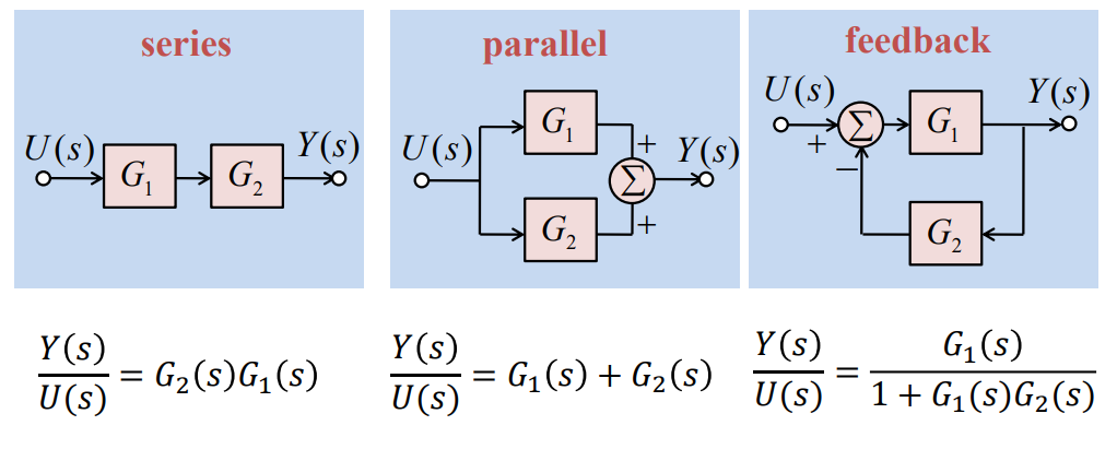
대부분의 시스템은 그것을 구성하는 서브시스템으로 분할할 수 있는데, 이때 각 서브시스템의 요소들은 서로에게 영향을 주지 않는다. 대신, 한 서브시스템의 출력이 다른 서브시스템의 입력으로 사용되고는 한다. 이 관계를 도식화하기 위한 툴이 바로 block diagram이다. Block diagram을 보면 전달함수를 쉽게 구할 수 있다.

Inverse Laplace Transform by partial fraction expansion

유리함수로 주어진 Laplace Transform은 partial fraction expansion과 inverse Laplace transform을 통해 time-domain 신호로 변환할 수 있다.

왜냐하면 우리는 \(\frac{1}{s+a}\)꼴과 \(\frac{as+b}{(s+c)^{2}+d^{2}}\)꼴의 inverse Laplace transform을 알고 있기 때문이다.

따라서 \(H(s)=K\frac{\prod_{i=1}^m(s-z_{i})}{\prod_{i=1}^n(s-p_{i})}=\sum_{i=1}^n\frac{k_{i}}{s-p_{i}}\)로 partial fraction expansion하여 inverse Laplace transform하면 h(t)를 구할 수 있다.

Initial Value Theorem & Final Value Theorem

라플라스 변환을 활용하면 time-domain에서의 초기값과 정상 상태에서의 값을 알 수 있다.

Initial Value Theorem: \(\lim_{t\to0} y(t)=\lim_{s\to\infty}sY(s)\)

Final Value Theorem: When all poles of \(sY(s)\) are on OLHP, \(\lim_{t\to\infty} y(t)=\lim_{s\to0}sY(s)\)

Time-domain Specification

Laplace transform을 통해 frequency response를 분석하지만, 결국 우리는 time-domain에 살고 있고 제어 또한 time-domain에서 이루어진다. 따라서 우리는 출력 신호가 time-domain에서 어떠한 응답을 가지는지 파악할 필요가 있고, 이때 사용하는 지표들이 time-domain specification이다. 대표적인 time-domain spec으로는 rise time, settling time, peak time, overshoot이 있다. 아래에는 각 spec의 정의와 second-order transfer function \(H(s)=\frac{\omega_{n}^{2}}{s^{2}+2\zeta\omega_{n}+\omega_{n}^{2}}\)에서 각 spec들을 근사적으로 구하는 방법을 소개한다.

Rise time

Rise time은 신호가 목표값의 10%~90% 구간에 머무는 시간을 의미하며, \(t_r\)로 쓴다. \(t_{r}\approx\frac{1.8}{\omega_n}\)이다.

Settling time

Settling time은 신호의 오차가 1% 이내로 유지되는 최단시간을 의미하며, \(t_s\)로 쓴다. \(t_{s}=\frac{4.6}{\sigma}\)이다.

Peak time

Peak time은 신호가 첫 피크에 도달하는 시간을 의미하며, \(t_p\)로 쓴다. \(t_{p}=\frac{\pi}{\omega_{d}}\)이다.

Overshoot

Overshoot은 최대 상대오차를 의미하며, \(M_p\)로 쓴다. \(M_{p}=e^{-\frac{\pi\zeta}{\sqrt{1-\zeta^{2}}}}\)이다.

Stability and Location of Poles

A LTI System is stable ↔ All poles are on OLHP

Poles on RHP make the system response diverge!

BIBO Stability

The system is BIBO stable: Bounded Input always makes a Bounded Output

The system is BIBO stable \(\Longleftrightarrow \int_{-\infty}^{\infty} |h(t)|dt <\infty\)

Proof

(i) ←:

\[|y(t)|=|\int_{-\infty}^{\infty}u(\tau)h(t-\tau)d\tau|\le \int_{-\infty}^{\infty}|u(\tau)h(t-\tau)|d\tau\le M\int_{-\infty}^{\infty}|h(t)|dt\]

(ii) →:

The statement is equal to: If \(\int_{-\infty}^{\infty} |h(t)|dt\) diverges, the system is not BIBO stable

Let \(u(t)=\begin{cases}1 && \text{if }h(t)>0 \\ -1 && \text{otherwise}\end{cases}\) then \(|y(t)|=|\int_{-\infty}^{\infty}u(\tau)h(t-\tau)d\tau|=|\int_{-\infty}^{\infty}|h(t-\tau)|d\tau|\) diverges, so the system is not BIBO stable

Routh Criterion

A LTI System is stable ↔ Every components in the first column of the Routh array is positive

What is the Routh Array?

Routh array is defined as:

\[\begin{pmatrix} 1 && a_{2} && a_{4} && \cdots \\ a_{1} && a_{3} && a_{5} && \cdots \\ b_{1} && b_{2} && b_{3} && \cdots \\ c_{1} && c_{2} && c_{3} && \cdots \\ \vdots && \vdots && \vdots && \\ * && * \\ * \\ *\end{pmatrix}\] \[b_{1}=-\frac{\text{det}\begin{bmatrix}1 && a_{2} \\ a_{1} && a_{3}\end{bmatrix}}{a_1}=\frac{a_{1}a_{2}-a_{3}}{a_{1}} \\ b_{2}=-\frac{\text{det}\begin{bmatrix}1 && a_{4} \\ a_{1} && a_{5}\end{bmatrix}}{a_1}=\frac{a_{1}a_{4}-a_{5}}{a_{1}} \\ b_{3}=-\frac{\text{det}\begin{bmatrix}1 && a_{6} \\ a_{1} && a_{7}\end{bmatrix}}{a_1}=\frac{a_{1}a_{6}-a_{7}}{a_{1}} \\ c_{1}=-\frac{\text{det}\begin{bmatrix}a_{1} && a_{3} \\ b_{1} && b_{2}\end{bmatrix}}{b_1}=\frac{b_{1}a_{3}-a_{1}b_{2}}{b_{1}} \\ c_{2}=-\frac{\text{det}\begin{bmatrix}a_{1} && a_{5} \\ b_{1} && b_{3}\end{bmatrix}}{b_1}=\frac{b_{1}a_{5}-a_{1}b_{3}}{b_{1}} \\ c_{3}=-\frac{\text{det}\begin{bmatrix}a_{1} && a_{7} \\ b_{1} && b_{4}\end{bmatrix}}{b_1}=\frac{b_{1}a_{7}-a_{1}b_{4}}{b_1} \\\]

We can expand the array in the same way.

The number of sign changes in the first column of the Routh array is equal to the number of poles on the RHP. Since the first component of the first column is positive(1), the first column should be positive.

Closed-loop system analysis

\[Y = GDR + GW\] \[E = (1-GD)R-GW\]

\[Y = \frac{GD}{1+GD}R+\frac{G}{1+GD}W-\frac{GD}{1+GD}V\] \[E = \frac{1}{1+GD}R-\frac{G}{1+GD}W+\frac{GD}{1+GD}V\]

Sensitivity

By some modeling error or environment change, plant G can change and thus transfer function T changes.

\[S = \frac{\text{fractional change in }T}{\text{fractional change in }G} = \frac{\frac{\delta T}{T}}{\frac{\delta G}{G}}\]

The system is robust when its sensitivity is low.

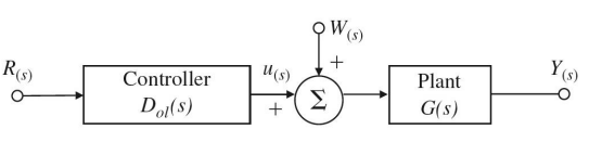
Sensitivity of open-loop system:

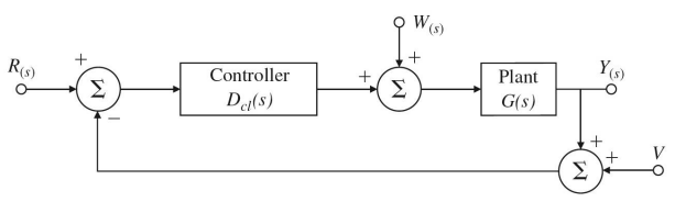
\[T+\delta T = D(G+\delta G) = DG +D\delta G=T+D\delta G\] \[\delta T = D \delta G, \frac{\delta T}{T}=\frac{D\delta G}{DG}=\frac{\delta G}{G}\] \[S = \frac{\frac{\delta T}{T}}{\frac{\delta G}{G}}=1\]

Sensitivity of closed-loop system:

using 1st-order approximation, \(\delta T =\frac{dT}{dG}\delta G\)

\[S =\frac{\frac{\delta T}{T}}{\frac{\delta G}{G}}=\frac{G}{T}\frac{\delta T}{\delta G}=\frac{G}{T}\frac{dT}{dG}=\frac{1}{1+GD}\]

System Type

Every inputs can be considered as polynomial inputs(according to Taylor expansion), and system with higher system type is able to maintain low steady-state error for high degree polynomial input.

System with system type n makes zero steady-state error for polynomial inputs with degree lower than n, nonzero finite steady-state error for polynomial inputs with degree n, infinite error for polynomial inputs with degree higher than n.

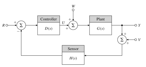
System type for reference tracking

\[E = \frac{1}{1+GD}R\]

System type n = number of poles of GD at the origin(s=0)

System type for disturbance rejection

\[E = -\frac{G}{1+GD}W\]

System type n = number of zeros of G/(1+GD) at the origin(s=0)

PID Control

\[u(t) = k_p e(t)+k_I\int_{t_0}^te(\tau)d\tau+k_D\frac{d}{dt}e(t)\] \[D(s)=k_p+\frac{k_I}{s}+k_Ds\]

Characteristic Equation of feedback system

\[T(s)=\frac{DG}{1+DGH}\]

Characteristic equation: \(1+D(s)G(s)H(s)=0\)→\(a(s)+Kb(s)=0\)→\(1+KL(s)=0\)

Pole of transfer function is a function of parameter \(K\)

What is Root Locus?

Root Locus is plot of the locus of all possible roots of \(1+KL(s)=0\) as \(K\) varies from \(0\) to \(\inf\)

How to draw the locus?

Just consider the rules.

\(L(s)=\frac{b(s)}{a(s)}\) and \(b(s)\), \(a(s)\) are monic polynomials with degree \(n,m (n\ge m)\)

Rule 1

The \(n\) branches of the locus start at the poles of \(L(s)\) and \(m\) of these branches end on the zeros of \(L(s)\)

Rule 2

The loci are on the real axis to the left of an odd number of poles and zeros

Rule 3

For large \(s\) and \(K\), \(n-m\) of the loci are asymptotic to the lines at angles \(\phi_l\) radiating out from the points \(s=\alpha\) on the real axis where

(angles of asymptotes) \(\phi_l = \frac{180^\circ+360^\circ (l-1)}{n-m}, l=1,2,\cdots,n-m\)

(center of asymptotes) \(\alpha = \frac{\sum p_i -\sum z_i}{n-m}\)

Rule 4

Angle of departure from a pole \(p_j\) of multiplicity \(q\):

\[q\phi_{l, \text{dep}}=\sum \psi_i-\sum \phi_i -180^\circ -360^\circ(l-1)\] \[\psi_i = \angle(p_j-z_i), \phi_i = \angle(p_j-p_i)\]

Angle of arrival at a zero \(z_j\) of multiplicity \(q\):

\[q\psi_{l, \text{arr}}=\sum \phi_i-\sum \psi_i +180^\circ +360^\circ(l-1)\] \[\psi_i = \angle(z_j-z_i), \phi_i = \angle(z_j-p_i)\]

Rule 5

The locus crosses the \(j\omega\) axis where the Routh criterion shows a transition from roots in the LHP to the roots in RHP.

If \(n-m>2\), at least one branch of the locus crosses the imaginary axis.

Rule 6

The locus has multiple roots at a point on the locus only if \(b\frac{da}{ds}-a\frac{db}{ds}=0\)

Argument Principle

A contour map of a complex function will encircle encircle the origin \(Z-P\) times clockwise, where \(Z\) is the number of zeros and \(P\) is the number of poles of the function inside the contour.

Nyquist Stability Criterion

By setting RHP as the contour, we can analyze stability of system with transfer function \(T(s) = \frac{KG(s)}{1+KG(s)}\)

We have \(Z=N+P\) where

\(Z\): the number of RHP poles of closed-loop system

\(N\): the number of clockwise encirclement of \(KG(s)\) about -1

\(P\): the number of RHP poles of open-loop system

Nyquist Plot

How to plot the Nyquist plot?

1. Plot \(KG(s)\) for the contour, which is a half circle with infinitely large radius
   1. Plot \(KG(s)\) for \(-j\infty \le s \le +j\infty\) (this can be done easily using Bode plot)
   2. If \(KG(s)=0\) at the origin, plot \(KG(s)\) for \(s=re^{j\theta}, (r=0, -\frac{\pi}{2}\le\theta\le\frac{\pi}{2})\)
   3. Plot \(KG(s)\) for \(s=re^{j\theta}, (r=\infty, -\frac{\pi}{2}\le\theta\le\frac{\pi}{2})\)
2. Evaluate the number of clockwise encirclement of -1 (=\(N\))
3. Determine \(P\)
4. \(Z=N+P\) and if \(Z=0\) the system is stable

Gain Margin and Phase Margin

Gain Margin

the factor by which the gain can be raised before instability results

\[GM =K^*/K\]

Phase Margin

the amount by which the phase of \(G(j\omega)\) exceeds -180 deg when \(|KG(j\omega)|=1\)

\[PM = \angle(KG(j\omega))-180 ^\circ\]